2 L'Opérateur Adjoint

A un opérateur linéaire continu $T:\mathcal{X}\longrightarrow \mathcal{Y}$ défini sur l'espace vectoriel normé $\mathcal{X}$ on peut associer un autre opérateur linéaire , appelé opérateur adjoint de $T$. On le note $T^{\times}$. L'intérêt pour cet opérateur est motivé par son utilité dans la résolution d'équations faisant intervenir des opérateurs. Citons les équations intégrales linéaires faisant intervenir des opérateurs compacts. De telles équations apparaissent de manière naturelle en physique. Dans cette section on définit l'opérateur adjoint,on démontre certaines de ses propriétés et on fait le lien avec l'opérateur adjoint $T^*$ dans le cas hilbertien. Il est important de préciser que cette discussion va dépendre du théorème 1.2.5 sans lequel rien ne serait ici possible.

On considère un opérateur linéaire continu $T:\mathcal{X}\longrightarrow \mathcal{Y}$ où $\mathcal{X}$ et $\mathcal{Y}$ sont des espaces vectoriels normés et on souhaite définir l'opérateur adjoint $T^{\times}$ de $T$. A cette fin on commence à partir de n'importe quelle fonctionnelle antilinéaire continue $g$ définie sur $\mathcal{Y}$, et on construit une une fonctionnelle antilinéaire continue $f$, définie sur $\mathcal{X}$ par

$$f(x)=g(Tx),\quad x\in\mathcal{X}.$$ (16)

$f$ est antilinéaire car $g$ est antilinéaire et $T$ est linéaire. $f$ est continue car bornée. En effet

$$\vert f(x)\vert=\vert g(Tx)\vert\leq\Vert g\Vert\Vert Tx\Vert\leq\Vert g\Vert\Vert T\Vert\Vert x\Vert.$$

Ainsi on obtient

$$\Vert f\Vert=\sup \{\vert f(x)\vert,x\in\mathcal{X}\ \Vert x\Vert=1\}\leq\Vert g\Vert\Vert T\Vert.$$ (17)

Ceci montre que $f\in\mathcal{X}^*$, l' adjoint de $\mathcal{X}$. Par hypothèse $g\in\mathcal{Y}^*$. Par conséquent, si $g\in\mathcal{Y}^*$ est vu comme variable, la formule (2.5) définit un opérateur agissant sur $\mathcal{Y}^*$ à destination de $\mathcal{X}^*$ qui est appelé l'opérateur adjoint de l'opérateur $T$ et noté $T^\times$. Ainsi on a $T^\times g=f$ rendant commutatif le diagramme (2.7)

$$\xymatrix @H=0pt{ \mathcal{X}\ar[rr]^T \ar[dr]_f & & \mathcal{Y}\ar[dl]^g \\ & {I\!\!K}& }$$ (18)

Opérateur Adjoint $T^×$. 2.1
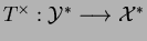
Soit $T:\mathcal{X}\longrightarrow \mathcal{Y}$ un opérateur linéaire continu, où $\mathcal{X}$ et $\mathcal{Y}$ sont des espaces vectoriels normés. Alors l'opérateur ajoint $T^\times:\mathcal{Y}^*\longrightarrow \mathcal{X}^*$ de $T$ est défini par

$$T^\times g=gT,\quad g\in \mathcal{Y}^*,$$ (19)

où $\mathcal{X}^*$ et $\mathcal{Y}^*$ sont les adjoints respectifs de $\mathcal{X}$ et $\mathcal{Y}$.

On va maintenant prouver que l'opérateur $T^\times$ est linéaire et a même norme que l'opérateur $T$. Cette démonstration nécéssitera l'emploi du théorème 1.2.5 qui dépend lui-même du théorème de Hahn-Banach.

Théorème. 2.2 (Norme de l'opérateur adjoint)
L'opérateur adjoint défini ci-dessus est antilinéaire continu et vérifie :

$$\Vert T^\times \Vert=\Vert T\Vert.$$ (20)

Proof.  
La linéarité de $T^\times$ provient directement du fait que son domaine d'application est l'espace vectoriel $\mathcal{Y}^*$. En effet on a pour tout $\alpha,\beta\in{I\!\!K}$, $g_1,g_2\in\mathcal{Y}^*$

$$\begin{array}{rcl} T^\times (\alpha g_1+\beta g_2)&=&(\alpha g_1+... ..._1\o T+\beta g_2\o T \\ &=&\alpha T^\times g_1+\beta T^\times g_2. \end{array}$$

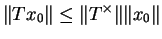
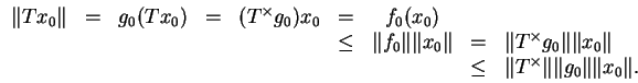
On va prouver (2.9) à partir de (2.8). Par l'inégalité (2.6) on a

$$\Vert T^\times g\Vert=\Vert f\Vert\leq\Vert g\Vert\Vert T\Vert.$$

En prenant dans cette inégalité le $\sup$ pour tout $g$ de norme $1$ on obtient

$$\Vert T^\times \Vert\leq\Vert T\Vert.$$ (21)

Pour obtenir (2.9), on doit maintenant prouver $\Vert T^\times \Vert\geq\Vert T\Vert$. Le théorème 1.2.5, appliqué relativement à l'espace $\mathcal{Y}$ et le diagramme (2.7) donnent maintenant que pour tout $x_0\in\mathcal{X}\backslash\ker(T)$, il existe un $g_0\in\mathcal{Y}^*$ tel que

$$\Vert g_0\Vert=1$$   et$$\qquad g_0(Tx_0)=\Vert Tx_0\Vert.$$

En fait ici $g_0(Tx_0)=(T^\times g_0)x_0$ par définition de l'opérateur adjoint $T^\times$. En posant $f_0=T^\times g_0$ on obtient

$$\begin{array}{rcccccccl} \Vert Tx_0\Vert & = & g_0(Tx_0) & ... ...& \Vert T^\times \Vert\Vert g_0\Vert\Vert x_0\Vert. \end{array}$$

Comme $\Vert g_0\Vert=1$ on a finalement

$$\Vert Tx_0\Vert\leq\Vert T^\times \Vert\Vert x_0\Vert$$   pour tout$$\ x_0\in\mathcal{X}.$$

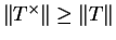
Ceci comprend $x_0\in \ker(T)$ car $T\ker(T)=\{0\}$. On a aussi l'inégalité

$$\Vert Tx_0\Vert\leq\Vert T\Vert\Vert x_0\Vert,$$

où $\Vert T\Vert=\inf\{c\geq 0 : \forall x_0\in\mathcal{X},\Vert Tx_0\Vert\leq c\Vert x_0\Vert\}$. Ainsi $\Vert T^\times \Vert$ ne saurait être plus petit que $\Vert T\Vert$. Donc

$$\Vert T^\times \Vert\geq\Vert T\Vert.$$ (22)

(2.11) et (2.10) donnent (2.9). $\qedsymbol$

On a les propriétés suivantes :
Soient $\mathcal{X},\mathcal{Y},\mathcal{Z}$ des espaces normés, $\alpha\in{I\!\!K}$, $T\in\L (\mathcal{X},\mathcal{Y})$ et $S\in\L (\mathcal{Y},\mathcal{Z})$, alors

$$(S+T)^\times = S^\times+T^\times$$ (23)

$$(\alpha T)^\times = \overline{\alpha} T^\times$$ (24)

$$(ST)^\times = T^\times S^\times$$ (25)

La propriété (2.14) se comprend aisément sur les diagrammes (2.15) et (2.16).

$$\xymatrix @H=0pt{ \mathcal{X}\ar[r]_T \ar@/^1pc/[rr]^{ST} & \mathcal{Y}\ar[r]_S & \mathcal{Z}\\ }$$ (26)

$$\xymatrix @H=0pt{ \mathcal{X}^* & \ar[l]_{T^\times} \mathcal{Y}^* &\ar[l]_{S^\times} \ar@/^1pc/[ll]^{T^\times S^\times} \mathcal{Z}^* }$$ (27)